ARM Frequently Asked Questions: Summarizing
How do I control the number of decimals for summary means in Summary reports?
How do I control the number of decimals for summary means in Summary reports?
By default, ARM reports one more decimal of accuracy on means than the most precise data point entered in a data column. For example, if the data points of 36, 45, and 98.02 are entered in a data column, ARM reports three decimals of accuracy on the means.
There are two methods to control or force the number of decimals accuracy.
Method 1
The easiest method is to use the 'Force Number of Decimals Accuracy to' option on the General Summary Report Options window. (General Summary report options apply to all summary reports.) Using this option, you may enter the number of decimals to use on summary reports when there is no entry for an assessment column in the assessment data header Number of Decimals field (see next paragraph).
Caution: Forcing number of decimals to 0 or 1 in General Summary Report Options is very likely to hide important differences for small treatment means, such as yield values less than 25.
Method 2
To override a default set by method 1, enter the number of decimals of accuracy desired in the Number of Decimals plot data header for each data column. Enter a "0" to force means to print as whole number with no decimals reported.
The number of decimals field is usually located at the bottom of plot data headers so you may have to scroll the data header window down to display this line. If some older GDM study definitions, it is the second entry field included on the same line as the number of subsamples. The data header prompt may appear as:
# Subsamples, Dec.
If you cannot see a number of decimals field on the plot data header, then check whether this field is hidden in the current Assessment Data View. Select Tools - Options then Assessment Data View, and be sure that Visible is checked for the Number of Decimals field.
Why do some treatment means have the same mean comparison letter when the difference between means is larger than the reported LSD?
Why do some treatment means have the same mean comparison letter when the difference between means is larger than the reported LSD?
Duncan's MRT, Student-Newman-Keuls, and Tukey's tests do not separate means the same as LSD. The mean comparison tests included in ARM are LSD, Duncan's MRT (called Duncan's New Multiple Range Test), Student-Newman-Keuls, Tukey's, Waller-Duncan, and Dunnett's. Mean comparisons based on LSD have often been criticized because the significance level "slips" when the number of treatments increases. (See 'AOV Means Table Report Options' in ARM Help for more information on mean comparison tests.)
If a group of treatment means are sorted in order from high to low, then Duncan's and LSD give approximately the same result for adjacent pairs of treatment means. (Adjacent pairs of treatment means are those beside each other when sorted in order from high to low.)
With Duncan's and Student-Newman-Keuls, the minimum value for significance becomes larger for mean pairs that are farther apart in the sorted list.
Both LSD and Tukey's use the same value for all tests, but the Tukey's value is quite large when compared to the LSD. (Thus, there are fewer significant differences.)
To use LSD as the mean comparison test in ARM (or to change mean comparison method):
To use LSD as the mean comparison test in ARM (or to change mean comparison method):
- Select File - Print Reports from the ARM menu bar.
- Double-click on the Summary heading in the left column that lists available reports to expand the list of available summary reports.
- Click once on AOV Means Table in the left column so this choice is highlighted.
- Click the Options button below the list of available reports to display the AOV Summary Report Options.
- Click the down pointing arrow following the mean comparison test method. Select LSD to use this test method.
- The F1 help also provides additional information on the mean comparison test methods.
Following is information about LSD extracted from 'AOV Means Table Report Options' in ARM Help:
When using LSD to make an unplanned comparison of the highest and lowest mean in a trial with more than two treatments, the difference between treatments can be substantial even when there is no treatment effect. For example, when using a 5% significance level the actual significance level is larger than 5%. Some statisticians have determined that for a trial with three treatments the significance level is actually 13%, for six treatments the significance level is 40%, for 10 treatments the significance level is 60%, and for 20 treatments the significance level is 90%.
[William G. Cochran and Gertrude M. Cox, Experimental Designs, 2nd edition (New York, John Wiley and Sons, Inc, 1957).]
There is also an AOV Means Table Report option set that is making "protected" mean comparison tests: the option to run mean comparison test "Only when significant AOV treatment P(F)". When this option is active, ARM will not report any differences as significant when the treatment probability of F is greater than the mean comparison significance level, for example 0.10 (or 10%). The statement that "Mean comparisons performed only when AOV Treatment P(F) is significant at mean comparison OSL." is printed as a report footnote when this option is active.
There is also an AOV Means Table Report option set that is making "protected" mean comparison tests: the option to run mean comparison test "Only when significant AOV treatment P(F)". When this option is active, ARM will not report any differences as significant when the treatment probability of F is greater than the mean comparison significance level, for example 0.10 (or 10%). The statement that "Mean comparisons performed only when AOV Treatment P(F) is significant at mean comparison OSL." is printed as a report footnote when this option is active.
Why do all treatment means have "a" as the mean comparison letter?
Why do all treatment means have "a" as the mean comparison letter?
Even though there may be considerable differences between treatment means, it is possible that ARM lists "a" as the mean comparison letter for all treatments for a particular column on the AOV Means Table report. This can occur when running a 'protected' mean comparison test, which is a statistically-recommended practice.
Selecting the option Only when significant AOV treatment P(F) on the AOV Means Table Report options enables the 'protected' mean comparisons. This means that if the AOV test statistic F is not significant (i.e. Treatment P(F) > signficance level), ARM will not perform mean comparisons. If this occurs, ARM will display the mean comparison symbol defined in the Symbol indicating no significant difference between treatment means AOV report option instead of the mean comparison letter. And if this option is blank, ARM displays 'a' beside all treatment means, which can appear as though a mean comparison was run with no differences found.
So, if all treatment means have "a" as the mean comparison letter even when it appears that differences should have been found, it is because the AOV treatment P(F) indicates that at the specified significance level, there is no statistical evidence supporting the AOV alternative hypothesis that "at least one treatment is different." Thus, there is no evidence to reject the null hypothesis that "all treatments are the same," and no reason to perform mean comparisons.
Why are treatment means of transformed data different than means of the original untransformed data?
Why are treatment means of transformed data different than means of the original untransformed data?
The reason there is a difference between the means of the transformed replicates when compared with the means of the raw data is because the means of transformed data are "weighted means". ARM performs Analysis of Variance on the transformed data values, calculates the treatment mean from the transformed values, then de-transforms the treatment means so they can be reported in the original units. (Means reported as log, square root, or arcsine percent values are very difficult to understand.)
The reason why the weighted means are different than the raw data means relates to the reason why the data must be transformed. A detailed explanation of the reason depends on which transformation was used.
Following is a description of the reason for this difference with data that has been transformed using square root. The description is from page 156 of the "Agricultural Experimentation Design and Analysis" book by Thomas M. Little and F. Jackson Hills, published 1978 by John Wiley and Sons. The discussion is regarding insect count data that was not normally distributed because many of the insect counts were very low - instead the data followed a Poisson distribution. The data was transformed and analyzed, means were calculated from the transformed values, then detransformed to the original units.
"The means obtained in this way are smaller than those obtained directly from the raw data because more weight is given to the smaller variates. This is as it should be, since in a Poisson distribution the smaller variates are measured with less sampling error than the larger ones."
Another way to say this is "The weighted means are more correct because the means are calculated from data where the original heterogeneity problem has been fixed."
What should I do if my data does not meet the assumptions of AOV?
What should I do if my data does not meet the assumptions of AOV?
There are several assumptions that the AOV analysis makes about the data in order to draw conclusions. The two assumptions that ARM tests for are:
- Normality – the distribution of the observations must be approximately normal, or bell-shaped. Simply put, most of observations will be relatively near the mean, so we can reasonably expect to not have major outliers. The measurements to test this assumption in ARM, which can be included on reports by selecting the respective AOV Means Table option, are:
- Skewness – a measure of how symmetrical the observed values are.
- Kurtosis – a measure of how ‘peaked’ the data is (how ‘flat’ or ‘pointed’ relative to the normal distribution).
- Homogeneity of variances – the variability of observations are approximately equal regardless of which treatment was applied. The mean comparison tests rely heavily on this assumption, since the tests are carried out using a common variance from all treatments. (Use “Bartlett’s Homogeneity of Variance” option on AOV Report Options to test for this assumption).
- The Box-Whisker graph is a great tool to visually investigate and demonstrate this concept. Boxes that are of similar height and shape across all treatments in a data column indicate homogenous variances.
If these assumptions are not met, the resulting analysis may be completely invalid:
“Failure to meet one or more of these assumptions affects both the level of significance and the sensitivity of the F test in the analysis of variance [AOV].” (Gomez and Gomez; Statistical Procedures for Agricultural Research pp.294-295).
There are a few things a researcher can try in order to “correct” the data to fit the assumptions of AOV. It should be stressed that these techniques are not “fudging” the data, but rather applying statistically-sound, industry-standard processes in order to compare the treatment means to get the mean comparison letters on the report. With ARM, these techniques can be automatically suggested using the option “Apply automatic transformations or treatment exclusions…” on the General Summary Report options.
- Apply automatic transformation – ARM can apply one of the following automatic data correction transformations:
- Square root (AS) – often used with ‘count’ rating types (e.g. # of insects per plant).
- Arcsine square root percent (AA) – used with counts taken as percentages/proportions.
- Log (AL) – can only be used for non-negative numbers.
The purpose of applying a transformation is to work with data that fits the assumptions of AOV – a transformation often fixes non-normality and/or non-homogeneity of variances by reducing the scale of the data. Note that it can be statistically and mathematically proven that:
“because a common transformation scale is applied to all observations, the comparative values between treatments are not altered and comparisons between them remain valid.” (Gomez and Gomez; Statistical Procedures for Agricultural Research pp.299)
Since the transformed data and resulting means will be on a different scale, use the “De-transform means” option on the General Summary report options to de-transform the means into the original units. Note that this does not affect any results.
- Exclude treatments – ARM can exclude a treatment from the analysis, most often to fix non-homogeneity of variances. Although this may not be desirable, as all treatments are included in the study for a reason, this option basically makes the best of a tough situation. Unless something is done to meet the assumptions of AOV, the entire study cannot be evaluated using AOV.
- ARM can apply the EC action code to exclude the check treatment. EC is often used for data where the untreated check plots are counts of weeds, while the other plots are a “% control” type of rating (thus a different rating type).
- ARM can apply the EC action code to exclude the check treatment. EC is often used for data where the untreated check plots are counts of weeds, while the other plots are a “% control” type of rating (thus a different rating type).
- Exclude Replicates – ARM can exclude a replicate from the analysis as well in order to meet the assumptions. Again, this is not desirable, but in certain cases is necessary in order to perform any analysis in ARM.
If none of the above correction techniques are able to fix non-normality and/or non-homogeneity of variances, the AOV analysis cannot be expected to be significant. Further statistical analysis will need to be performed in order to draw conclusions from the data.
How does ARM calculate the Standard Deviation for the AOV Means Table report?
How does ARM calculate the Standard Deviation for the AOV Means Table report?
By definition, standard deviation is the square root of variance. The standard deviation reported by ARM is the square root of the Error Mean Square (EMS) from the AOV table. When trial data is analyzed as a randomized complete block (RCB), ARM performs a two way analysis of variance (AOV). As a result, both the treatment and the replicate sum of squares are partitioned from the error sum of squares.
Sometimes a user attempts to verify the standard deviation calculated in ARM by using a spreadsheet or a scientific calculator. It is important to note that the standard deviation calculated by a spreadsheet or a scientific calculator is typically based on a one way AOV. The EMS (and thus the standard deviation) calculated for a one way ANOVA is different than that calculated for a two way AOV, so standard deviation calculated by ARM for a RCB experimental design will almost always be different than the standard deviation calculated using a spreadsheet or scientific calculator. In other words, the variance (EMS) is not the same when calculated for a two way ANOVA as a one way ANOVA.
ARM performs a one way AOV only when analyzing trial data as a completely random experimental design. For a completely random design, the standard deviation calculated by Excel or a scientific calculator will match the one calculated by ARM.
What is the difference between Bartlett's and Levene's tests of homogeneity of variance?
What is the difference between Bartlett's and Levene's tests of homogeneity of variance?
On the AOV Means Table report, select the 'Homogeneity of variance test' descriptive statistic to print a test statistic and the significance level for the selected test of homogeneity of variance. The significance indicates the likelihood that data violates the assumption of homogeneity of variance. Thus, a probability of 0.05 indicates a 95% certainty that variances are heterogeneous.
When the data is reasonably normally-distributed, Levene's and Bartlett's tests are comparable, with a slight edge to Bartlett's. (Use the Skewness and Kurtosis statistics to test for normality.)
- If you have strong evidence that your data do in fact come from a normal, or nearly normal, distribution, then Bartlett's test has more statistical power.
However, Levene's test is less sensitive to departures from normality than Bartlett's. So if the Bartlett's test fails for a given column, it could be due to non-normality or heterogeneity of variance. But without evidence that the data is nearly normal, you cannot be certain that it is the heterogeneity of variance that the test is detecting.
- Thus when the data is non-normal or skewed, Levene's test provides better results.
Therefore Levene's test is the recommended option overall.
Reference:
Milliken and Johnson. Analysis of Messy Data. Chapman & Hall/CRC, 1992.
Dose-Response Analysis Report
Dose-Response Analysis Report
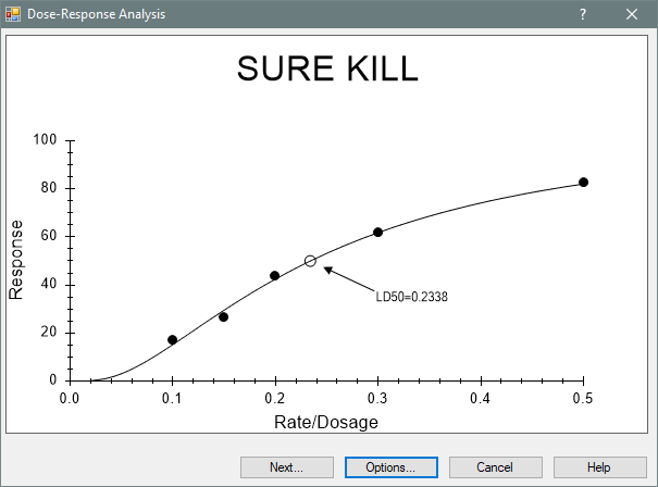
The dose-response analysis is used in experiments where a treatment or chemical is applied at different rates, and the level of response to the dosage is recorded (as a percentage or count of individuals that responded). The analysis estimates the treatment rate/dosage that results in a response from a particular percentage of individuals in the study. One example is the LD50, which estimates the dosage level that results in a response of 50%, i.e. the median lethal dose.
ARM provides three different Dose-Response estimation algorithms: Probit - Least Squares, Probit - Maximum Likelihood, and Logit. These algorithms were provided courtesy of Dr. J. J. Hubert, University of Guelph.
See Dose-Response Analysis Report (pdf) for information about printing this report.